Part I: Statistical Process Control — Getting Down to Basics

Statistical process control is a valuable tool that helps users understand, monitor, and control manufacturing processes. This article presents a comprehensive look at SPC. In Part I, the author introduces the concept of SPC and how it relates to quality, advantages of implementing SPC, and statistical concepts such as variation, distribution, standard deviation, subgroups, and quality characteristics. Part II will delve deeper and discuss the control charts and their interpretation, control and specification limits, quality charts for variable and attribute data, and process statistics.

By Jodi Kay, Quality Engineer, SPSS Inc.

Statistical process control — or SPC — goes hand in hand with quality. In order to understand the benefits and reasons for using SPC, one should have a basic knowledge of quality concepts. Quality can be defined as the degree to which products or services conform to a defined standard or specification.

Quality of products or services can be broken down into two categories, design quality and conformance quality. Design quality is a measure of the extent to which a product's or service's design specifications actually reflect the customer's needs and requirements. Conformance quality describes the consistency to which the product or service meets the design requirements. Without design quality a product or service could be produced consistently but still will not meet the customer's needs. On the other hand, if a product or service is high in design quality and low in conformance quality, it, too, will not satisfy the customer needs. The technique of SPC is used to manage conformance quality.

In the past, quality professionals tried to "inspect" quality into their products. They would inspect 100% of the products and separate the conforming parts from the non-conforming ones. Inspection was performed after the product was manufactured. The conforming parts would be shipped to the customer while the non-conforming parts were either reworked or scrapped. There were a number of problems with this technique. First, it was costly and time-consuming to inspect every product. Also, some non-conforming products would inadvertently get accepted as conforming and be shipped to the customer. Finally, there were significant costs associated with reworking and scrapping materials. However, to ensure quality, users of SPC sample a specified number of products at defined intervals during the manufacturing process instead of 100% inspection after manufacturing.

Defining SPC
SPC is a quality tool that uses statistical theories for monitoring a process to ensure statistical control in order to improve consistency. The term statistical process control can be broken down. "Statistical" means drawing conclusions using an analytical, qualitative approach to interpret data. A "process" is a combination of people, equipment, materials, and environment working together to produce an identifiable, measurable output. And "control" involves making something behave in a consistent, predictable manner.

The methodology is based on statistical theories and rational sampling and can be applied to two types of data: variable, which is measured, and attribute, which is counted.

Some distinct reasons for using SPC are:

• to identify and eliminate the special causes of variation

• to measure the size of common cause variation and determine if it is small enough to yield acceptable results

• to increase communication between operators and management

• to decrease the recurrence of problems

SPC also helps reduce the costs of quality, which are associated with producing products or providing services that don't conform to requirements. Costs can be incurred internally from increased process times and raw material costs due to scrapping and reworking materials. Other costs are associated with customer dissatisfaction as a result of receiving non-conforming products or late shipments.

Variation and Other Statistical Concepts
SPC is used to monitor variation. Variation is inevitable and occurs in everything. No two items are identical. For example, if we measure the length of two pencils manufactured from the same process that were supposed to be 3 in., we'd find that one can be 2.95 in. and another 3.18 in. Both pencils would not be exactly 3 in. If we measured 30 more pencils from that process, we'd find that they would also vary in length. The amount of variation detected would be a function of the device used to measure the length. If these measurements were plotted by frequency of occurrence, they would form a probability distribution curve.

Probability Distributions
There are many different types of probability distribution curves that a set of measurements can form. A probability distribution is a mathematical formula that relates the values of the characteristic with the probability of occurrence in the population. It can fall into two categories: continuous or discrete. A probability distribution is continuous if the characteristic being measured is a real number that can be of any value (subject to the degree of certainty of the measurement equipment). These types of measurement characteristics are called variable data (the length of a pencil is a variable characteristic). A probability distribution is discrete if the characteristic being measured can be only specific integer values (0, 1, 2, 3). Attribute characteristics fall into this category. SPC assumes variable data falls into the most common of the continuous probability distribution types, the bell-shaped curve or normal distribution.

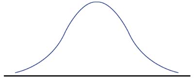
Normal Distribution
The normal distribution has the shape of a bell, hence it's often referred to as the bell-shaped curve.

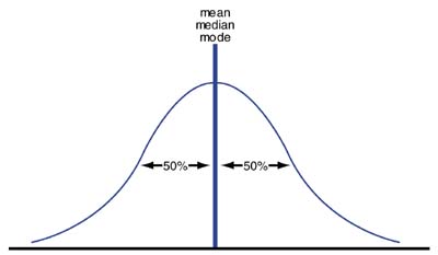
The highest point on the curve represents the mean, medium, and mode (in a normal distribution these values are all equal). Mean, medium, and mode are all measures of central tendency (where a process is targeted). The curve is symmetrical, therefore, one could draw a vertical line from the highest point on the bell-shaped curve to the bottom (the horizontal axis) and 50% of the values would fall on either side of this vertical line. (See Figure 2.)

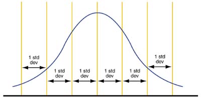
The symmetry is an advantage of the bell-shaped curve. The curve can be divided into six equal areas, each comprised of one standard deviation, as shown in Figure 3. Standard deviation, a measure of dispersion or variation, quantifies the amount of spread inherent in a data set or how much a data point deviates from the mean. If there's a lot of variation, the standard deviation will be large. The larger the standard deviation, the wider the normal distribution. This indicates more fluctuation of data, thus, the data is less predictable.

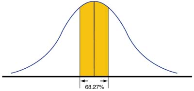
The first two areas of the bell-shaped curve we will consider are ±1 standard deviation from the mean. A significant percentage of the data will fall in this area, or 68.27%.

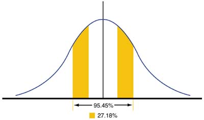
A less significant percentage of data fall into the areas between ±1 standard deviation and 2 standard deviations from the mean, 27.18%. Collectively, ±2 standard deviations from the mean make up 95.45% of the data.

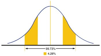
Finally, 4.28% of the data falls in the areas of the curve between two and three standard deviations from the mean. In this case, ±3 standard deviations from the mean make up 99.73% of all of the data. Therefore, if a set of measurements is normally distributed, it's highly improbable that a point belonging to that normal distribution will fall outside of ±3 standard deviations from the mean.

Normal distribution is useful because it allows us to predict where data will fall in respect to the mean. To ensure data is normally distributed, we can measure (when applicable) more than one part during a sampling. This group of measurements taken at a point in time is referred to as a subgroup. The reason for measuring more than one part at a time is due to the central limit theorem.

In other words, during a sampling, if we use a subgroup size greater than 1, then no matter what probability distribution that subgroup belongs to, we can approximate it as a normal distribution and draw the same conclusions. The larger the subgroup size, the closer the subgroup will approach a normal distribution.

Editor's Note: Part II of this article will cover how to use and interpret charts, discuss control and specification limits, quality charts for variable and attribute data, and process statistics. Readers who have questions or comments can send them to me at nkatz@metrologyworld.com. I will forward them to the author.

Reference
1. Quality with Confidence in Manufacturing, Jeffrey T. Luftig, Ph.D.

About the Author
Jodi Kay has been working as a quality engineer for SPSS Inc. since joining the company in 1996. She currently works on special projects for the Quality in Manufacturing group. Kay received her bachelor's degree in industrial and systems engineering from Ohio University in 1990, and is finishing up her MBA at Depaul University. Since graduating from Ohio University, she has been employed at Com-Corp. Industries, Carbide International, and Ferro Corp. as a quality engineer.